Block/Bidding Evaluation
Overview
The Bidding Forecast uses statistical models of 25 variables (such as proximity to existing leases, previous bids, newly available, etc.)...
Input
The forecast requires these user supplied parameters...
Output
Zip file containing...
Methodology
The area of interest is restricted to deep water blocks, blocks in water with a depth greater than 656 ft. (200 meters)....
Results
Estimated probabilities...
Overview
The Bidding Forecast uses statistical models of 25 variables (such as proximity to existing leases, previous bids, newly available, etc.) to estimate both the likelihood of a block being bid in the next sale (bid/no-bid) but also an estimated bid amount. The analysis is run on companies individually except a group of small companies who have had few bids or little money exposed recently in deep water..
Input
The forecast requires these user supplied parameters:
- Training Period (At least 3 years are required).
- Price of Oil.
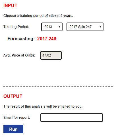
Output
Zip file containing:
- Primary Report (PDF reviewing the methodology, analysis of resulting probabilities of being bid and forecasted bid amount, and analysis of influential factors for each company).
- MROV Report (PDF reviewing the methodology for the MROV forecast)
- Feature Class of results (Bid/No-Bid Probability, Forecasted Bid Amount, Minimum MROV Probability, Forecasted MROV).
- Text Files of results (csv).
- Feature Class of Bid Attributes used to make the forecast.
- Fully specified models.
- Confidence intervals on the forecast.
- Full analysis on blocks not available in the sale (this is primarily current leases).
Methodology
Area of Interest
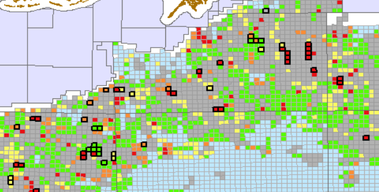
The area of interest is restricted to deep water blocks, blocks in water with a depth greater than 656 ft. (200 meters). Only blocks near current leases are forecasted. Near is defined as the 95th percentile of bidding distances to current leases, historically. This is about two blocks away from any current lease. Additionaly blocks that were rejected within one year or blocks near discovered fields are included in the area of interest. Most blocks beyond the area of interest have very little relevant, publicly available data and are unlikely to receive bids. While training the model, the same restrictions are used.
List of Bidding Attributes
| Variable Type | Variable | Description |
|---|---|---|
| Global | Region | Western vs. Central |
| Water Depth | Block's water depth | |
| Oil Price ($2017) | Oil price at the time of the sale in real 2017 dollars | |
| Change in Oil Price (t-(t-1)) | Percent difference of oil price at the time of forecast sale and oil price of last prior sale | |
| Local | Open Blocks | Density of open blocks |
| Field EUR | Averaged estimated ultimate recovery of nearby fields | |
| Discoveries | Density of nearby discoveries | |
| Wells | Density of wells | |
| Platforms | Distance to the nearest platform | |
| First Time Availability | Is the block a first time available block | Local Company Specific | Past Leases | Density of past leases |
| Current Leases | Density of current leases | |
| Relinquished Undrilled Leases | Density of relinquished undrilled leases | |
| Relinquished Drilled Leases | Density of relinquished drilled leases | |
| Bid Amounts | Weighted (by time and distance) past bid amounts | |
| High Bid Amounts | Weighted (by time and distance) past high bid amounts | |
| Lost Bids | Density of bids where another company won | |
| Rejected Bids | Density of bids that were rejected by BOEM | MROV | Platforms | Distance to the nearest platform |
| Years Unleased | The number of years unleased | |
| First time availablity | Is this the first sale this block is available? | |
| Average Proximate MROV | The average MROV of immeditaly surrounding blocks weighted by time. | |
| Relinquishments | Is the lease available because it was relinquished? | |
| Proximate Leases | How many immediatly proximate leases surround the block. | |
| Recent MROV | The most recent MROV on the block. | |
| EUR of Nearby Field | The EUR of the nearest field | |
| Rejections | Was the field rejected the last time it was bid on? | |
| Discoveries | The number of nearby discoveries. |
List Of Companies
High-activity and medium-activity companies are modeled individually and low-activity companies are modeled as a group.
| Activity | Company |
|---|---|
| High - Activity | Shell, Statoil, ExxonMobil, Chevron, BP, BHP, Anadarko |
| Medium - Activity | Hess, Cobalt, Llog, Venari, Ecopetrol, Noble, Murphy, Stone, Red Willow, Apache, Repsol, Ridgewood, Total, Houston Energy |
| Low - Activity | Nexen, Petrobras, Eni, Woodside, Deep Gulf, Navitas, Enven, Talos, Tana Exp., MCX, Nippon, Gulfslope, Walter, Fieldwood, Focus, Rising Natural Resources, Arena, W&T, Calypso, ATP Oil&Gas, Davis Offshore, Energy Resource Tech, Wild Well, Dynamic Offshore, CL&F, and all others. |
Forecast Models
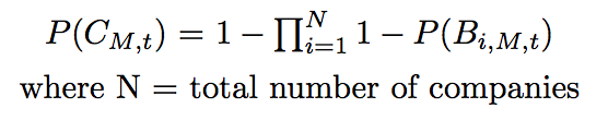
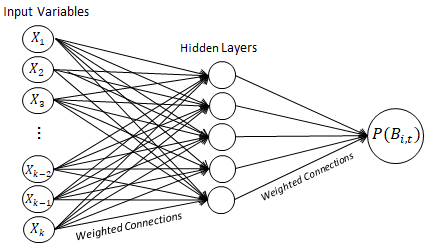
BID/NO-BIDLogistic regression is used as the statistical method. The candidate explanatory variables include global, local, and company specific variables. The final output is represented as P(BM,i,t), the probability of block, M, being bid by company, i, at time, t. Additionally, a block can be generalized to all companies, which is represented as P(CM,t),the probability of at least one company bidding on block, M, at time, t.
Linear regression is used as the statistical method. The candidate explanatory variables are the global and local variables. Company specific variables are excluded due to the small sample size of blocks bid by each company per sale. This does not give an estimated bid amount per company, just the estimated high bid amount. The final output is represented as YM,t, the predicted high bid amount conditional on block, M, being bid by a company at time, t.
Minimum MROV Likelihood
A random forest model is used to predict the likelihood a block will receive a minimum MROV (currently $576,000). All the MROV variables are used in this model. The output is the likelihood that the block will be a minimum MROV.
MROV Amount
A random forest model is used to forecast the MROV assigned by the government. The same variables as the Minimum MROV likelihood model are used here. The output is the predicted MROV amount. Since the majority of blocks are assigned a minimum MROV, only blocks that have less than an 80% chance of being a minimum MROV are forecasted with this model. The blocks with greater than an 80% chance of being a minimum MROV are simply assigned $576,000.
Additional Model Details
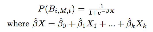
LOGISTIC REGRESSION FOR BID/NO-BID
Logistic Regression analyzes the outcome of a qualitative, dependent variable based on the effects of the Xk independent explanatory variables. Logistic regression is implemented twice to model bid/no-bid. The first implementation considers all variables tht have little to no correlation with one another. The second implementation includes only the variables considered "statistically significant" in the first implementation. The final model is represented through the following equation. This equation follows a logistic, S-shaped curve.
Multiple Linear Regression develops a model that predicts a quantitative, dependent variable based on the effects of the Xk independent explanatory variables. In order to find the optimal model, the "stepwise" selection method is used for variable selection. The stepwise method iteratively builds the model by adding or removing variables based on it's significance and overall performance of the model. The final model is represented through the following linear eqution.
![]()
Random forest is a machine learning technique that is used for classification and regression. In a nutshell, it creates many decision trees (hence the name) and averages the results to get its predictions. It was chosen for MROV predictions because it handles unbalanced data very well. The majority of blocks receive the minimum MROV so this method handles the imablance well. The largest downside is interprebility (there are no coefficients like in regression that tell you the magnitude of influence) but we do have variable importance plots included in the MROV report.
Results
Estimated Probabilities
The probability scores for all blocks are binned into 5 different cohorts from A (highest likelihood of being bid) to E (lowest likelihood of being bid). The bins are made by dividing the cummulative probability by percentiles. The top 5% of cummulative probabilties are assigned A blocks, 5%-15% are assigned B, 15%-30% C, 30%-50% D and the bottom 50% are assigned E. Note that since the probabilities are not uniformly distributed, there many more than 50% of the blocks will receive the E category. For each cohort, a short term and long term probability is calculated. Short term is defined as blocks bid during the forecast period and long term is defined a blocks bid in the following 3 years. The short and long term errors are given in the bidding report.